The Maximum Likelihood Estimate

After choosing a distribution to model your data, point estimates of the distribution’s parameter(s) can be derived based on what the most likely value(s) would maximize the likelihood function of interest.

Note that a likelihood function is not the same as a probability function. A likelihood function is defined as the probability that we observe a set of data given a set of values of the a parameter. So the value of the parameter is a variable that determines the probability in question (i.e. it is a function of the parameter). In contrast, this same parameter is not a variable in the probability function and the area under this curve must sum to 1 whether the function is discrete or continuous. It is a function of the set of data.

In terms of the calculations, the likelihood function is equivalent to the probability we observe a set of data for all values of a given parameter in its parameter space. We often make the assumption that the data were independent and identically distributed (i.i.d.), so this calculation simply boils down to multiplying the probabilities together. This is an example of frequentist statistics, where probabilities are calculated with no prior knowledge of the data. This is contrasted by Bayesian statistics.

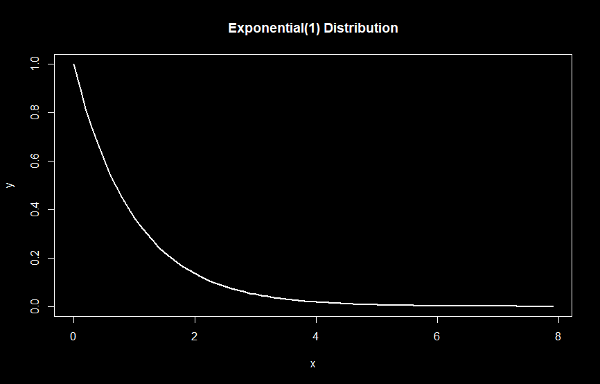
Let’s take a look at an example with the exponential distribution. The figure below depicts an Exponential(1) distribution plotted in R, which has one parameter, often referred to as the rate parameter.

As mentioned previously, the likelihood function is a function of the parameter (in this case, the rate parameter). In the case of an Exponential(1) distribution, it is intuitive that the maximum likelihood estimate is the rate itself (in this case, 1). This can also be derived by solving for the value of the parameter that equates the log of the derivative of the likelihood function to zero. Essentially, we are solving for the argmax of the maximum value of the likelihood function by finding points where its slope is zero. The log likelihood function is usually used to simplify this calculation. Note that this method of finding the maximum likelihood estimate may not always work; numerical methods such as Newton’s method will need to be used in this case.

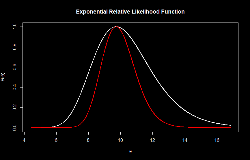
In the figure below we plot the relative likelihood (white curve) and log relative likelihood (red curve) functions in R. It is easy to see why we can use the log of the likelihood function to solve for the maximum likelihood estimate - the value that maximizes the probability is equal in both cases; taking the log does not change the estimated parameter.