The Machine Learning Pipeline

The goal of this article is go over the many steps of the machine learning process at a high level, from data collection to deploying the model to the web.

1. Collecting the Data

The first part of any machine learning project is to collect relevant data. What problem are we trying to solve? Is the data public? Where will we store the data? Is the data structured or unstructured? Structured data can contain categorical, numerical, ordinal, or times series data, and it’s important to distinguish each.

2. Exploratory Data Analysis

After we’ve collected our data, we need to establish the target variable and our features to better understand what we’re working with. Our dataset will likely have missing values and/or outliers, and there are many different approaches to handling those. We can choose to impute missing values with the mean, median, or even remove those entries altogether. For outliers, we can scale all our values or just remove them. It all depends on the nature of our data and how much of it we have.

To simplify this process, it is a good idea to create plots. There are many Python and R libraries such as matplotlib, seaborn, or plotly that make it easy to create beautiful visuals. Below are examples of plots I’ve created while exploring the data in a drug classification problem.

Sample visuals of feature distributions in a drug classification problem

3. Data Preprocessing

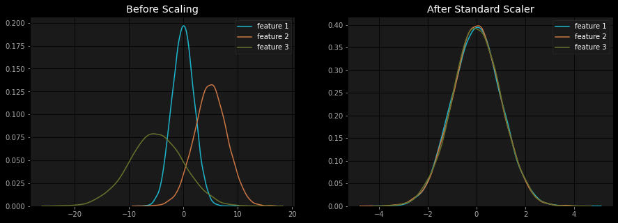
Now it’s time to prepare our data to be modelled. If we have categorical features, we need to encode them. If our numerical features are on very different scales (e.g. one feature ranges from 0-10 while another ranges from 100-1000), we should apply some form of scaling to normalize the values. For example, standard scaling subtracts the mean from each value and divides by the standard deviation, leaving the features with a mean of 0 and a standard deviation of 1.

Applying standard scaling to sample features

At this point it is important to solidify our understanding of the features instead of blindly feeding the values to a model. This will allow for effective feature engineering, as it will help us identify useful ways to modify our features and create new ones. For example, if one of our features was a datetime, it may be useful to create a new feature that specifies what day of the week that was.

Selecting which features to use is the next step. If we have a lot of them, we may want to reduce the dimensionality with techniques such as Principal Component Analysis. In future steps when we analyze our model, we may need to come back to this step and drop features that were found to be less important.

Next we need to split our data into training, validation, and test sets. Holding out parts of our data will help give us an idea of how our model will perform in the real world and also help avoid overfitting. The ratios for the split will depend on how much data you have and how balanced it is.

4. Choosing an Algorithm

There are many supervised and unsupervised algorithms commonly used in machine learning. Choosing which to use will depend on the type of problem (i.e. regression, classification) and the target outcome. For example, we may choose to use linear regression if the outcome was a continuous variable and logistic regression when predicting a binary outcome. Other common supervised algorithms include K-Nearest Neighbours, Support Vector Machines, decision trees/random forests, neural networks, and more.

5. Hyperparameter Tuning

This section is essentially adjusting the right parameters to optimize our model’s performance. Perhaps the most important hyperparameter is the learning rate. Some machine learning libraries such as Tensorflow and scikit-learn have built in optimizers for neural networks that will automatically tune the learning rate over a certain number of epochs. Depending on the type of model, there will be different hyperparameters to tune (e.g. maximum depth of tree-based models, or number of layers in a deep neural network).

Accuracy and Loss vs. Epochs for a CNN model trained with the Adam Optimizer

6. Evaluating the Model

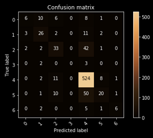
Choosing what metric to evaluate our model on will depend on the type of problem. Regression models tend to be evaluated on the (root) mean squared error, mean absolute error, or its R-squared value. Classification models are typically evaluated on accuracy, precision, recall, or its f1 score. Together, these components can be combined to produce a confusion matrix like the one below.

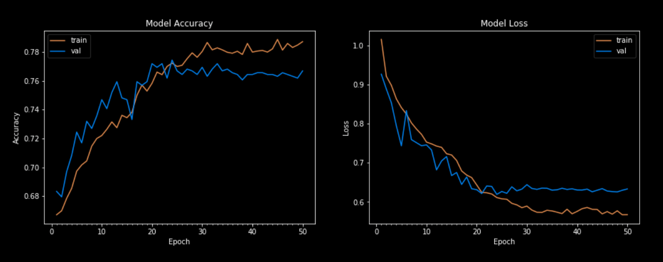
There are also some important considerations to take into account during this stage. Is the model underfitting/overfitting the data? Is there any correlation in the predictions that my model is getting wrong? How do all my models compare? Based on these findings, it may be worthwhile to go back to previous steps and adjust accordingly.

7. Deploying the Model

The final step is to serve our model to the web. We should continue to evaluate our model against real world data and make the necessary changes based on how it performs. The model may need to be retrained over time as new and updated data becomes available.

Summary

And that’s it! This was a very high level overview of an end to end machine learning project. Each stage can be further broken down into much more detail, but the aim of this article was just to provide a general idea of what the pipeline looks like.